Solving a Kaggle ML classification problem using XGBoost
- 21 minsThis post is about my first ever participation in a kaggle competition. The competition was organized by the Machine Learning techers of the MSc course I’m currently doing. To be honest, I had no idea about how to get through this kind of competition, but since it was a mandatory assignment and I had to do it, me and my colleague really spent a lot of time trying to get the best possible score. All the details about the classification problem can be found in kaggle, and the whole implementation of the model can be found in this public repo.
Disclaimer:
This post is not intended to show a rigurous and very formal approach of the problem solving, actually is intended to do the complete opposite. I will try to show how me and my colleague tackled the problem when knowing almost nothing in machine learning and how we obtained a score higher than 99%. For a more formal-ish approach of the work you can take a look at the report we wrote.
Summary
Below, there is a summary of the whole pipeline. On the next blocks, we will dive deeply in all the modules shown.
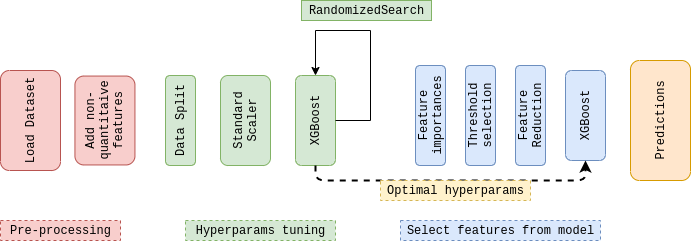
Pre-Processing
The Dataset
The dataset has been obtained from a real LTE deployment. During two weeks, different metrics were gathered from a set of 10 base stations, each having a different number of cells, every 15 minutes. The dataset is provided in the form of a csv file, where each row corresponds to a sample obtained from one particular cell at a certain time. Each data example contains the following features:
-
Time: hour of the day (in the format hh:mm) when the sample was generated. -
CellName: text string used to uniquely identify the cell that generated the current sample. CellName is in the form xαLTE, where x identifies the base station, and α the cell within that base station (see the example in the right figure). -
PRBUsageULandPRBUsageDL: level of resource utilization in that cell measured as the portion of Physical Radio Blocks (PRB) that were in use (%) in the previous 15 minutes. Uplink (UL) and downlink (DL) are measured separately. -
meanThrDLandmeanThrUL: average carried traffic (in Mbps) during the past 15 minutes. Uplink (UL) and downlink (DL) are measured separately. -
maxThrDLandmaxThrUL: maximum carried traffic (in Mbps) measured in the last 15 minutes. Uplink (UL) and downlink (DL) are measured separately. -
meanUEDLandmeanUEUL: average number of user equipment (UE) devices that were simultaneously active during the last 15 minutes. Uplink (UL) and downlink (DL) are measured separately. -
maxUEDLandmaxUEUL: maximum number of user equipment (UE) devices that were simultaneously active during the last 15 minutes. Uplink (UL) and downlink (DL) are measured separately.maxUE_UL+DL: maximum number of user equipment (UE) devices that were active simultaneously in the last 15 minutes, regardless of UL and DL. -
Unusual: labels for supervised learning. A value of 0 determines that the sample corresponds to normal operation, a value of 1 identifies unusual behavior.
# Clone repository in order to get access locally to the datasets
!rm -rf .git README.md
!git clone https://github.com/sergio-gimenez/anomaly-4G-detection
train = pd.read_csv('anomaly-4G-detection/ML-MATT-CompetitionQT2021_train.csv', sep=';')
test = pd.read_csv('anomaly-4G-detection/ML-MATT-CompetitionQT2021_test.xls', sep=';' )
# Separate labels from data
X = train.drop('Unusual', axis='columns')
y = train['Unusual']

# We split the data into training and validation subsets (80% and 20%) in
# order to validate our training
X_train, X_validation, y_train, y_validation = train_test_split(X, y,
                                                                train_size=0.8,
                                                                random_state=1, stratify = y)
X_test = test
Using non-quantitative features
First thing to do regarding data pre-processing is to make sure all
features are ready to be used, specially the non numerical ones: Time
and CellName. Time has relevant correlation with the maximum traffic
hours, although the day is not included in the date, still is a relevant
enough feature. In order to make Time ready to use, there are several
approaches. However, the chosen one has been to convert the time
(minutes) to radians and split them up into two features, one applying a
cosine and the other with sine. Regarding CellName, a simple mapping
1:1 with a numerical identifier for each cell name has been carried out.
#Refactor time feature to minuts and cellName to unique identifier 1:1
def getTimeInMinutes(x):
  hh, mm  = x.split(":")
  return int(hh)* 60 + int(mm)

def createCellNameDictionary(data):
  cellList = []
  for i in data["CellName"]:
    cellList.append(i)
  cellList = set(cellList)
  cellDict = {}
  for idx, value in enumerate(cellList):
    cellDict[value]=idx
  return cellDict

def refactorFeaturesDataframe(data):
  #data["Time"] = data["Time"].apply(lambda x: getTimeInMinutes(x))
  data["TimeCos"] = data["Time"].apply(lambda x: math.cos(getTimeInMinutes(x)*math.pi/(12*60)))
  data["TimeSin"] = data["Time"].apply(lambda x: math.sin(getTimeInMinutes(x)*math.pi/(12*60)))
  del data["Time"]

  cellNameDict = createCellNameDictionary(data);
  data["CellName"] = data["CellName"].apply(lambda x: cellNameDict[x])
  return data
#Refactoring data from features to useful values
X_train_df = refactorFeaturesDataframe(X_train)
X_train = X_train_df.to_numpy()
y_train = y_train.to_numpy()
X_validation = refactorFeaturesDataframe(X_validation).to_numpy()
y_validation = y_validation.to_numpy()
X_test = refactorFeaturesDataframe(test).to_numpy()
Data Visualisation
PCA
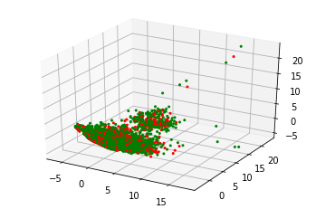
Regarding PCA, given the number of new features desired, it tries to provide the projection using the correlation between some dimensions and keeping the maximum amount of information about the original data distribution. As can be seen in the image below, there are not clear clusters nor a clear defined pattern. Usual and unusual samples are mixed in many ways, fact that constraints the classifier that is going to be used, e.g linear classifiers can be directly excluded.
pca = PCA(n_components=3)  # Reduce to k=3 dimensions
scaler = StandardScaler()
X_norm = scaler.fit_transform(X_train)
X_reduce = pca.fit_transform(X_norm)

colors=['green' if l==0 else 'red' for l in y_train]
fig = plt.figure()
ax = fig.add_subplot(111, projection='3d')
ax.scatter(X_reduce[:,0], X_reduce[:, 1], X_reduce[:, 2], s=4, alpha=1,color=colors)
plt.show()
t-SNE
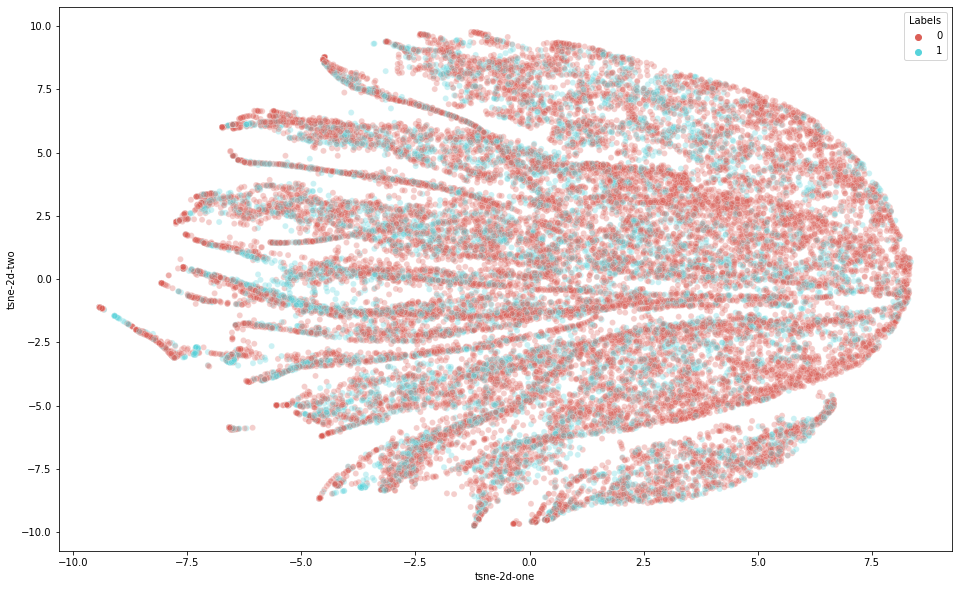
In order to go through a different approach, a non-linear reduction such as t-SNE has been tried out. t-SNE is an unsupervised method that minimizes the divergence between a distribution that measures pairwise similarities of the input and a distribution that measures the similarities of the corresponding low-dimensional points in the embedding. As it can be observed in the figure below, t-SNE has built a set of separable clusters but with samples of different classes mixed in the same clusters, without a clear visual pattern.
from sklearn.manifold import TSNE
tsne = TSNE(n_components=2, verbose=1, perplexity=40, n_iter=300)
tsne_results = tsne.fit_transform(X_train)

df_subset={}
df_subset['tsne-2d-one'] = tsne_results[:,0]
df_subset['tsne-2d-two'] = tsne_results[:,1]
df_subset['Labels'] = y_train

plt.figure(figsize=(16,10))
sns.scatterplot(
    x="tsne-2d-one", y="tsne-2d-two",
    hue="Labels",
    palette=sns.color_palette("hls", 2),
    data=df_subset,
    legend="full",
    alpha=0.3
)
Plain Vanilla Classifiers
Due to the dataset nature, a linear classifier will not achieve an acceptable performance. A neural network did not work either due to the small dataset. A SVM with a Gaussian kernel was tested as well but, the results were not as good as the ones obtained by decision tree. Some results applying plain vanilla classifiers without any parameter tuning are shown in the table below. As it can be seen, the best performance is obtained with a plain vanilla decision tree. Therefore, we decided to dive deeply into that approach.
| Classifier | Train Err. | Valdiation Err. | Accuracy |
|---|---|---|---|
| Decision Tree | 0 | 0.03 | 0.96 |
| SVM (rbf) | 0.26 | 0.26 | 0.73 |
| MLP | 0.27 | 0.27 | 0.73 |
Solving the Classification Problem
XGBoost. Training the classifier
One of the widely ensembled methods are gradient boosted decision trees.
In a summarized way, boosting takes an iterative approach for training
models. It trains models in succession, with each new model being
trained to correct the errors made by the previous ones. A widely used
implementation of the training described before is XGBoost. XGBoost
is an optimized distributed gradient boosting library designed to be
highly efficient, flexible and portable.
All the necessary information about XGBoost can be found in the
XGBoost Documentation Page
Note:
If you want to avoid the training process, and use the pre trained
model, make sure the xgb_model.joblib is loaded in
anomaly-4G-detection/xgb_model.joblib.
If you want to go through the training process there are two ways:
-
Fast way: The most suitable parameters we have found are already hardcoded in the pipe and no training process is involved at all in this part.
-
Whole training process: If you want to do the whole training process by yourself comment the parameters in the pipe, comment
clf_GS = RandomizedSearchCV(estimator=pipe, param_distributions=parameters, n_jobs=10, verbose=1, cv=[(slice(None), slice(None))], n_iter= 1)and uncomment
clf_GS = RandomizedSearchCV(estimator=pipe, param_distributions=parameters, n_jobs=10, verbose=1, cv=5, n_iter= 500)
from xgboost import XGBClassifier, plot_importance
from joblib import dump, load
from google.colab import files
from scipy.stats import uniform, randint

try:
  clf_GS = load('anomaly-4G-detection/xgb_model.joblib')
  training = False

except:
  training = True
  pipe = Pipeline(steps=[('std_slc', StandardScaler()),
                         ('xgb_clf', XGBClassifier(random_state=1,
                                                      scale_pos_weight=7,
                                                      colsample_bytree= 0.053381469489678104,
                                                      eta= 0.20289460663803338,
                                                      gamma= 0.88723107873764,
                                                      learning_rate= 0.15455380920536027,
                                                      max_depth= 26,
                                                      min_child_weight= 1,
                                                      n_estimators= 565,
                                                      subsample= 0.9738168894035317))])

  parameters = {
  # 'xgb_clf__eta'    : uniform(0.2, 0.35),
  # "xgb_clf__colsample_bytree": uniform(0.05, 0.2),
  # "xgb_clf__min_child_weight": randint(1, 5),
  # "xgb_clf__gamma": uniform(0.35, 0.6),
  # "xgb_clf__learning_rate": uniform(0.1, 0.3), # default 0.1
  # "xgb_clf__max_depth": randint(10, 30), # default 3
  # "xgb_clf__n_estimators": randint(500, 1000), # default 100
  # "xgb_clf__subsample": uniform(0.6, 0.99)
  }

  #clf_GS = RandomizedSearchCV(estimator=pipe, param_distributions=parameters, n_jobs=10, verbose=1, cv=5, n_iter= 500)
  clf_GS = RandomizedSearchCV(estimator=pipe, param_distributions=parameters, n_jobs=10, verbose=1, cv=[(slice(None), slice(None))], n_iter= 1)
  clf_GS.fit(X_train, y_train)
Select features from model
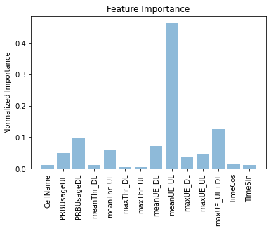
The last experiment that leads to a considerable enhancement is to take
advantage of the features selected by the model to perform a feature
reduction. Take into account that XGBoost, in essence, is a set of
ensemble decision trees, so we could evaluate its features importance
once the model is trained.
Evaluating that data, we get the optimized threshold to reduce the accuracy using just 3 features (check next code block). The ‘SelectFromModel’ module allowed us to pass the thresholds to the already trained model and, once the best threshold is validated, transform the datasets using just the features that pass the threshold. This final experiment let us reduce the recall from 44 errors in validation to 14. In the test set we achieved a score of 99.83%, which was our best performance in the challenge.
from sklearn.feature_selection import SelectFromModel

if training:

  treshold_train_error = []
  treshold_val_error = []
  thresholds = np.sort(clf_GS.best_estimator_.named_steps["xgb_clf"].feature_importances_)

  current_error = 100.0
  best_th = 0

  for thresh in thresholds:

    # Do a feature reduction with relevant feature
    new_X_train = X_train
    selection = SelectFromModel(clf_GS.best_estimator_.named_steps["xgb_clf"], threshold=thresh, prefit=True)
    select_X_train = selection.transform(new_X_train)

    # Fit the classifier with the reduced dataset
    selection_model = RandomizedSearchCV(estimator=pipe, param_distributions=parameters, n_jobs=10, verbose=1, cv=[(slice(None), slice(None))], n_iter= 1)
    selection_model.fit(select_X_train, y_train)

    # Evaluate predictions with the dataset trained with the feature reduction
    pred_train = selection_model.predict(select_X_train)
    select_X_val = selection.transform(X_validation)
    pred_val = selection_model.predict(select_X_val)


    """"
         Classification report
         ---------------------
    """
    train_error = 1. - accuracy_score(y_train, pred_train)
    train_cmat = confusion_matrix(y_train, pred_train)
    val_error = 1. - accuracy_score(y_validation, pred_val)
    val_cmat = confusion_matrix(y_validation, pred_val)

    treshold_train_error.append(train_error)
    treshold_val_error.append(val_error)

    print("\nThreshold of value %f" % thresh)
    print("--------------------------------")
    print('\ntrain error: %f ' % train_error)
    print('train confusion matrix:')
    print(train_cmat)
    print('\ntest error: %f ' % val_error)
    print('test confusion matrix:')
    print(val_cmat)
    print("\n")

    if val_error < current_error:
      current_error = val_error
      best_th = thresh
      best_transformation = select_X_train
Train and predict the data with the best feature reduction
  from sklearn.feature_selection import SelectFromModel

  # Get the best estimator we found in the previous block
  new_X_train = X_train
  selection = SelectFromModel(clf_GS.best_estimator_.named_steps["xgb_clf"], threshold=best_th , prefit=True)
  select_X_train = selection.transform(new_X_train)

  # Train the classifier with the best feature reduction
  selection_model = RandomizedSearchCV(estimator=pipe, param_distributions=parameters, n_jobs=10, verbose=1, cv=[(slice(None), slice(None))], n_iter= 1)
  selection_model.fit(select_X_train, y_train)

  # Save the model in a file and download locally.
  dump(clf_GS, 'xgb_model.joblib')
  files.download('xgb_model.joblib')

  pred_train = selection_model.predict(select_X_train)
  select_X_val = selection.transform(X_validation)
  pred_val = selection_model.predict(select_X_val)

  train_error = 1. - accuracy_score(y_train, pred_train)
  train_cmat = confusion_matrix(y_train, pred_train)
  val_error = 1. - accuracy_score(y_validation, pred_val)
  val_cmat = confusion_matrix(y_validation, pred_val)


  """"
         Classification report
         ---------------------
  """

  print("\nThreshold of value %f" % thresh)
  print("--------------------------------")
  print('\ntrain error: %f ' % train_error)
  print('train confusion matrix:')
  print(train_cmat)
  print('\ntest error: %f ' % val_error)
  print('test confusion matrix:')
  print(val_cmat)
  print("\n")

  print("TRAINING\n" + classification_report(y_train, pred_train))
  print("\nTESTING\n" + classification_report(y_validation, pred_val))
And the results of the best estimator:
Threshold of value 0.462643
--------------------------------

train error: 0.000034
train confusion matrix:
[[21376     1]
 [    0  8146]]

test error: 0.002439
test confusion matrix:
[[5340    4]
 [  14 2023]]


TRAINING
              precision    recall  f1-score   support

           0       1.00      1.00      1.00     21377
           1       1.00      1.00      1.00      8146

    accuracy                           1.00     29523
   macro avg       1.00      1.00      1.00     29523
weighted avg       1.00      1.00      1.00     29523


TESTING
              precision    recall  f1-score   support

           0       1.00      1.00      1.00      5344
           1       1.00      0.99      1.00      2037

    accuracy                           1.00      7381
   macro avg       1.00      1.00      1.00      7381
weighted avg       1.00      1.00      1.00      7381
Insightful data visualization
Here, there is some data visualisation in order to see and understand why and what improved by performing the feature reduction.
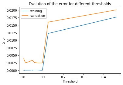
Evolution of the error for different thresholds
This plot shows the improvement we gained by implementing the ‘Feature Selection’ module.
  fig, ax = plt.subplots()
  ax.plot(thresholds, treshold_train_error, label='training')
  ax.plot(thresholds, treshold_val_error, label='validation')
  ax.set(xlabel='Threshold', ylabel='Error')
  ax.legend()
  plt.title('Evolution of the error for different thresholds')
  plt.show()
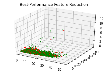
Best performance feature reduction
Our best feature reduction has 3 features , so then we can plot the resulting data set.
  colors=['green' if l==0 else 'red' for l in y_train]
  fig = plt.figure()
  ax = fig.add_subplot(111, projection='3d')
  ax.scatter(best_transformation[:,0], best_transformation[:, 1], best_transformation[:, 2], s=4, alpha=1,color=colors)

  plt.title('Best-Performance Feature Reduction')
  plt.show()
Feature importance
In this plot, is shown the features that are more relevant to XGBoost when it comes to classify.
  feature_importances = clf_GS.best_estimator_.named_steps["xgb_clf"].feature_importances_
  columns = X_train_df.columns

  fig = plt.figure()
  plt.bar(np.arange(14) , feature_importances, align='center', alpha=0.5)
  plt.xticks(np.arange(14), columns, rotation='vertical')
  plt.ylabel('Normalized Importance')
  plt.title('Feature Importance')
  plt.show()
Conclusions
During this research, we have explored a vast amount of possible classifiers and techniques to deal with the binary classification problem exposed in this report. Among those all classifiers, XGBoost has resulted to be the proper one to perform this task, as other related resources suggested.
References
Some nice references we checked in order to solve the problem:
- XGBoost Documentation
- How to Use XGBoost for Time Series Forecasting
- XGBoost model
- Python Hyperparameter Optimization for XGBClassifier using RandomizedSearchCV
- A Beginner’s guide to XGBoost
- The proper way to use Machine Learning metrics
- XGBoost and Imbalanced Classes: Predicting Hotel Cancellations

Sergio Giménez Antón
Passionate about networks, coding, travelling and hiking